本篇博客的主要内容有:
- 逻辑回归理论知识
- python代码实现EX2的第一个练习
这篇博客的主要来源是吴恩达老师的机器学习第三周的学习课程,还有一些内容参考自黄海广博士的笔记GitHub,先根据作业完成了matlab代码,并且学习将它用python来实现(博客中无matlab实现)。在学习的过程中我结合吴恩达老师的上课内容和matlab代码修改了一部分代码(个人认为可以优化的地方)。
逻辑回归总结
Logistic Regression for Classification
线性回归不适合用来解决分类问题,因为分类问题不是一个线性函数,加入新的样本,就可能导致线性回归的方程改变了,使得我们没有办法找到正确的划分点,因此没有办法分类。
线性回归问题其$h_{\theta}(x)$的值可能是大于1或者小于0的
而对于分类问题,我们的输出只有0或者1(二分类),因此$h_{\theta}(x)$太大或者太小都不行,我们可以用逻辑函数(logistic function,也可以叫做sigmoid函数)来使$0\leq h_{\theta}(x) \leq 1$
不要被回归所误导,逻辑回归解决的是分类问题
Hypothesis Representation
逻辑回归模型的 $h_\theta(X)=g(\theta^{T}X)$
$X$ 代表特征向量
$g$ 代表逻辑函数(logistic function)是一个常用的逻辑函数为S形函数(Sigmoid function),公式为: $g(z)= \frac{1}{1 + e^{-z}}$
这里有个概念非常重要,那就是:
$h_\theta(X)$ = estimated probability that y=1 on input x
也就是说,经过sigmoid函数作用后的$h_\theta(X)$,输出的是y=1的概率!
也就是说:
$h_\theta(X) = P(y=1 | x;\theta)$
Decision boundary
我们假设,
$h_\theta(X) \geq 0.5$时 y=1 也就是$\theta^{T}X \geq 0$
$h_\theta(X) < 0.5$时 y=0 也就是$\theta^{T}X < 0$
这里的等号不需要纠结
也就是说$\theta^{T}X = 0$就是我们的决策边界
对于简单的线性可分的边界,我们可以直接画出来一条直线
对于复杂的比如不能非线性可分的,我们可以通过添加多项式项,得到更加复杂的决策边界
Cost Function
如果我们和线性回归一样,定义代价函数为:
$J\left( {\theta_{0}},{\theta_{1}}…{\theta_{n}} \right)=\frac{1}{2m}\sum_{i=1}^{m}(h_{\theta }(x^{(i)})-y^{(i)})^{2}$
那么将我们的$h_\theta(X)$ (非线性函数 non-linear function)代入,将会得到一个非凸函数,有许多的局部最小值,我们使用梯度下降就不能保证收敛到全局最小值,如下图所示: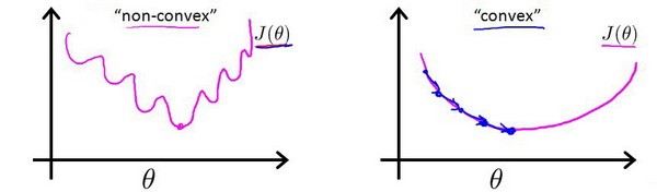
因此我们的代价函数定义为:
$J_{\theta} = \frac{1}{m}\sum_{i=1}^{m}cost(h_{\theta}(x^{(i)}),y)$
其中
$cost(h_{\theta}(x),y)=\left\{\begin{matrix}
-log(h_{\theta}(x)) .. if..y=1
\\
-log(1-h_{\theta}(x)) .. if ..y=0
\end{matrix}\right.$
下图画出了cost的图像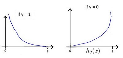
下面我们讨论这个公式的意义
y = 1时
- cost = 0 if y = 1,$h_{\theta}(x)=1$
但是 当$h_{\theta}(x)=1 \rightarrow 0$时,$cost \rightarrow \infty $ - 也就是: if $h_{\theta}(x)=0$(预测$P(y=1|x;\theta) =0$,但是实际上样本分类为y=1,这样我们将进行惩罚,penalize learning algorithm by a very large cost
同理 y=0(样本正确分类是0)时,当$h_{\theta}(x)=1 \rightarrow 0$时,预测$P(y=1|x;\theta) =1$,$cost \rightarrow \infty $(设置无穷大的cost)
总结下,就是下面的意思(可以结合上面的图像来看):
$cost=0, if h_{\theta}(x) = y$
$cost \rightarrow \infty, if y=0 and h_{\theta}(x) \rightarrow 1$
$cost \rightarrow \infty, if y=1 and h_{\theta}(x) \rightarrow 0$
这样我们通过减少cost,就能找到目标$\theta$啦
同时我们这里的cost能够保证$J(\theta)$是凸函数(NG老师貌似讲了一个极大似然估计然后说是凸的,这里我是一只鸵鸟跳过)
下面是cost的简单写法:
$cost = -y^{i}log(h_{\theta}(X^{(i)}))-(1-y^{i})log(1-h_{\theta}(x^{(i)}))$
可以验证y=1或者0代入时就是刚刚前面的cost
那么我们有
$J(\theta) = \frac{1}{m}\sum_{i=1}^{m}[-y^{i}log(h_{\theta}(X^{(i)}))-(1-y^{i})log(1-h_{\theta}(x^{(i)}))]$
其梯度定义为:
$\frac{\partial J(\theta)}{\partial \theta_{j}} = \frac{1}{m}\sum_{i=1}^{m}(h_{\theta}(x^{(i)})-y^{(i)})x_{j}^{(i)}$
求偏导数的求导过程如下,比较麻烦我直接贴图,不用markdown公式了,不过推导起来难度不大。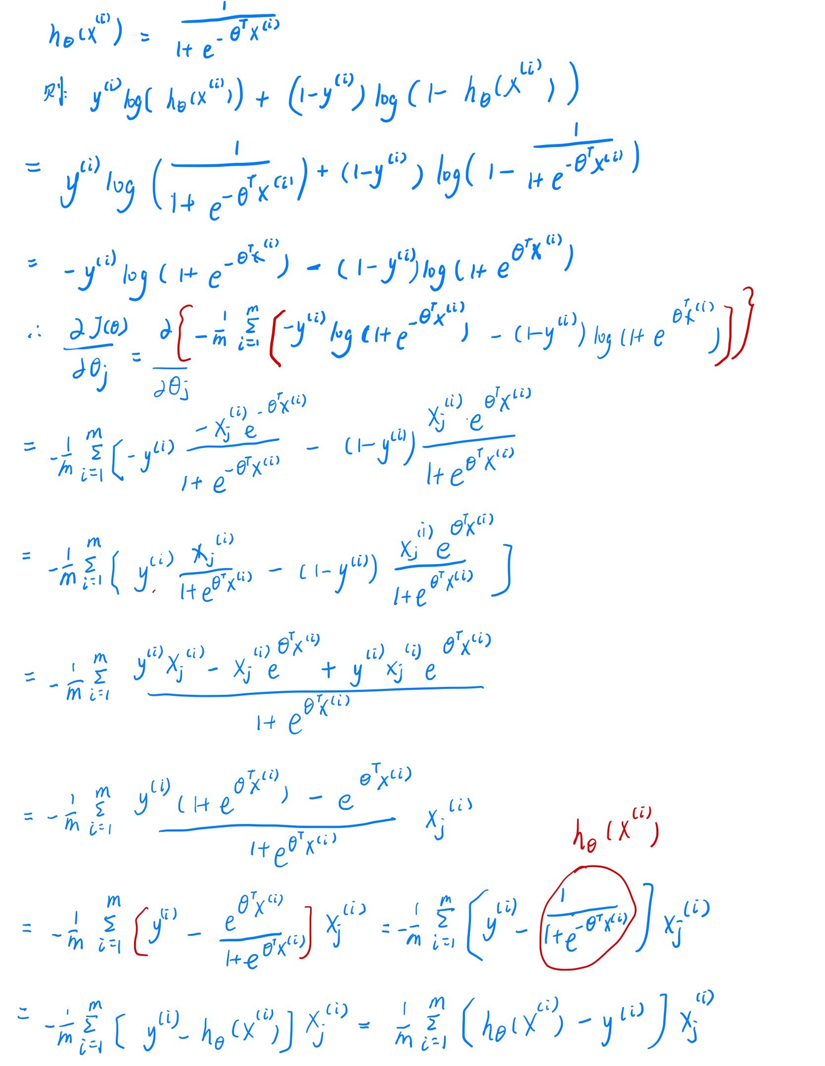
算出来梯度后,我们会发现,逻辑回归和线性回归的梯度是一样的形式,但是由于$h_{\theta}(x)$是不一样的,所以梯度是不一样的(这可能就是为啥叫逻辑回归的原因?)
接下来我们就可以使用梯度下降法来优化$\theta$了。
梯度下降法的向量化写法
在实际的代码实现中,我们一般把每个特征写成行向量(n个维度),m个样本组成了$X_{m \times n}$矩阵,我们会将$\theta$写成列向量$\theta_{n \times 1}$
这样有
$h = g(X\theta)$
$J_{\theta} = \frac{1}{m}\sum_{i=1}^{m}[-y^{i}log(h_{\theta}(X^{(i)}))-(1-y^{i})log(1-h_{\theta}(x^{(i)}))]$
Grandient Descent:
repeat{
$\theta_{j} := \theta_{j} - \alpha \cdot \frac{\partial J(\theta)}{\partial \theta_{j}} $
}
其中
$\frac{\partial J(\theta)}{\partial \theta_{j}} = \frac{1}{m}\sum_{i=1}^{m}(h_{\theta}(x^{(i)})-y^{(i)})x_{j}^{(i)})$
更新$\theta$的向量化表示:
$\theta := \theta - \frac{\alpha}{m} \cdot X^{T} \cdot (g(X\theta)-\vec{y})$
使用matlab或者python的优化算法来优化$\theta$
梯度下降法是一种常用的优化算法,但是还存在其他的优化算法如:
Gradient descent- Conjugate gradien
- BFGS
- L-BFGS
相比较梯度下降,这些算法的有点在于:
- 不需要我们人工的选择$\alpha$
- 通常会比梯度下降计算的快
但是这些Advanced optimization也更加复杂,算法的性能与实现的好坏有关系
这些算法理解起来难度比较大,但是这些复杂的理论就交给数学家们去研究吧,我们当一只鸵鸟,会用即可,不需要知道其内部实现
Multi-class classification One-Vs-All
对于多分类问题,我们可以每次将一类样本当作一类,其他所有样本当作另外一类,c类样本的话总共需要c个分类器,当我们用来预测时,只需要将新的样本输入,然后选择c个分类器中概率最大的那个
训练逻辑回归分类器$h_{\theta}^{(i)}(x)$
对于每一类$i$ 来预测$y=i$的概率
对新的$x$,我们有$class = max_{i}(h_{\theta}^{(i)}(x))$
下面是具体的代码实现
python代码实现
读入数据并可视化
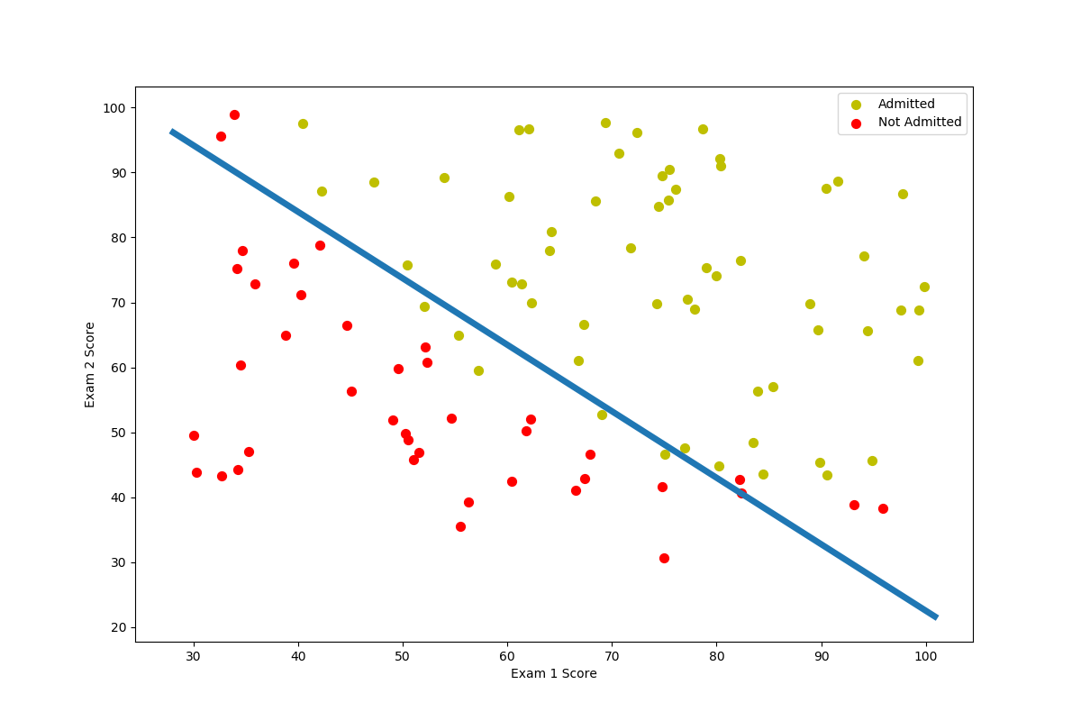
学生两次考试的成绩和最后是否被录取的结果来训练回归模型(分类),再用它来做预测。
先读入数据,并且输出数据前几行
1
2
3
path = 'ex2data1.txt'
data = pd.read_csv(path,header=None,names=['Exam 1','Exam 2','Admitted'])
print(data.head())找到分类为1和分类为0的,并用不同颜色将他们画出来
1
2
3
4
5
6
7
8
9
10
11
12
13
def plotData(positive,negative):
fg,ax = plt.subplots(figsize = (12,8))
ax.scatter(positive['Exam 1'],positive['Exam 2'],s=50,c='y',marker='o',label='Admitted')
ax.scatter(negative['Exam 1'],negative['Exam 2'],s=50,c='r',marker='o',label='Not Admitted')
ax.legend()
ax.set_xlabel('Exam 1 Score')
ax.set_ylabel('Exam 2 Score')
plt.show()
positive = data[data['Admitted'].isin([1])]
negative = data[data['Admitted'].isin([0])]
plotData(positive,negative)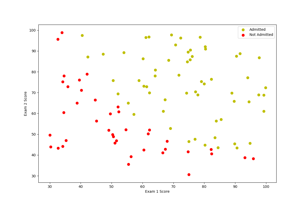
仔细观察图像,这两类样本之间存在清晰的决策边界,因此我们可以训练逻辑回归模型。
sigmoid函数
$h_\theta(X)=g(\theta^{T}X)$
$g(z)= \frac{1}{1 + e^{-z}}$
其代码实现为:1
2def sigmoid(z):
return 1/(1+np.exp(-z))我们可以画出sigmoid函数的图像来看看我们的函数是否写的正确:
1
2
3
4
5def checkSigmoid():
fig,ax = plt.subplots(figsize=(12,8))
nums = np.arange(-10,10,step=0.1)
ax.plot(nums,sigmoid(nums),'r')
plt.show()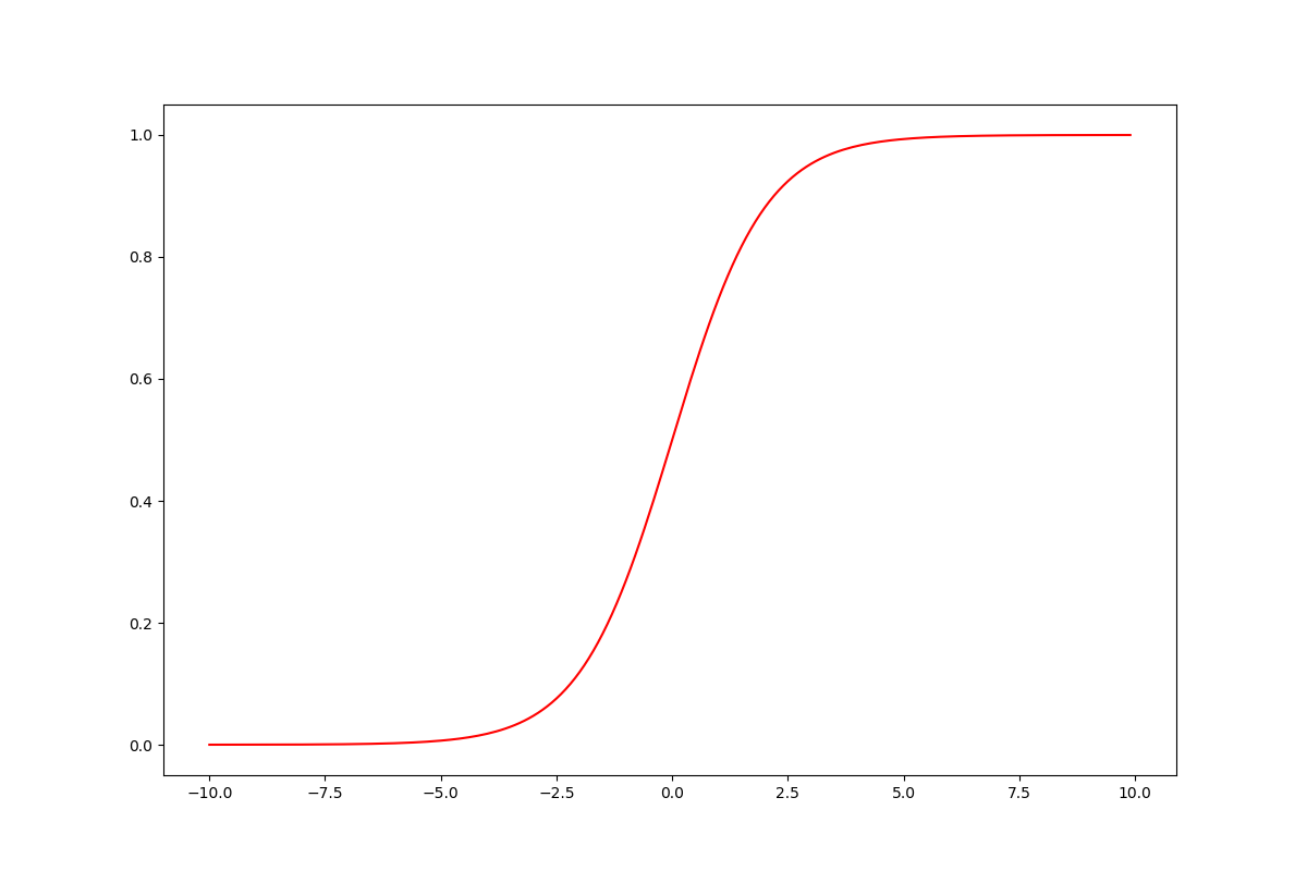
从图像来看,我们的sigmoid函数写的是没有问题的
计算代价函数和梯度
$J_{\theta} = \frac{1}{m}\sum_{i=1}^{m}[-y^{i}log(h_{\theta}(X^{(i)}))-(1-y^{i})log(1-h_{\theta}(x^{(i)}))]$
$\frac{\partial J(\theta)}{\partial \theta_{j}} = \frac{1}{m}\sum_{i=1}^{m}(h_{\theta}(x^{(i)})-y^{(i)})x_{j}^{(i)})$
1 | def costFunction(theta,X,y): |
定义完这两个函数,我们设置数据,进行验证1
2
3
4
5
6
7data.insert(0, 'Ones', 1)
cols = data.shape[1]
X = data.iloc[:,0:cols-1]
y = data.iloc[:,cols-1:cols]
X = np.array(X.values)
y = np.array(y.values)
theta = np.zeros(3)
这里是直接使用numpy的array数组,因为在后面使用python的优化函数时候,遇到了维数问题报错((100, 1)和(100,),我建议别转成矩阵,直接用array来计算
Basically you are running up against the fact that np.matrix is not fully supported by many functions in numpy and scipy that expect an np.ndarray. I highly recommend you switch from using np.matrix to np.ndarray - use of np.matrix is officially discouraged, and will probably be deprecated in the not-too-distant future.可以看这个解释
1 | print(costFunction(theta,X,y),gradFunction(theta,X,y)) |
调用函数后,出现下面的结果,就说明我们计算代价函数和梯度的代码没有问题了(第一个是$J_{\theta}$,第二个是$\frac{\partial J(\theta)}{\partial \theta_{j}}$1
2
3
4[0.69314718]
[[ -0.1 ]
[-12.00921659]
[-11.26284221]]
优化$\theta$
在NG老师的练习中,是使用一个称为“fminunc”的Octave函数是用来优化函数来计算成本和梯度参数。由于我们使用Python,我们可以用SciPy的“optimize”函数来优化。
1 | import scipy.optimize as opt |
上面的opt函数有一些注意点:
- costFunction和gradFunction这两个函数的定义上注意先让theta在前面,再定义参数X,y,下面的x0是传入我们初始的$\theta$,我们的目标就是要找到最优的$\theta$,让$J_{\theta}$最小
- 最后的args就是我们前面应该要传入cost和grad函数的参数
- 注意维度问题(前面已经提过,我建议使用array,不一定非要用matrix)
- 返回值中第一个就是我们的目标$\theta$
上面的代码执行后,应该是下面的结果:1
2(array([-25.1613186 , 0.20623159, 0.20147149]), 36, 0)
[0.2034977]
其中上面第二行是使用优化后的$\theta$计算的$J_{\theta}$
接下来我们就可以使用$\theta$画出决策边界了:
决策边界是一条直线,我们只需要输入两个端点,即可画出直线
这里X坐标取得是X数据中x1的最大值或者最小值+-2
Y坐标的话是根据
$h_{\theta}(X) = \theta_{0} + \theta{1}x_{1} + \theta{2}x_{2}$来推得:
$x_{2} = \frac{ -\theta_{0}-\theta{1}x_{1}}{\theta{2}}$
$x_{2}$就是我们点的Y坐标1
2
3
4
5
6
7
8
9
10
11theta_min = result[0]
pointX = np.array([np.min(X[:,1])-2,np.max(X[:,2])+2])
pointY = (- theta_min[0] - theta_min[1] * pointX)/theta_min[2]
fig,ax = plt.subplots(figsize=(12,8))
ax.plot(pointX,pointY,linewidth=5)
ax.scatter(positive['Exam 1'],positive['Exam 2'],s=50,c='y',marker='o',label='Admitted')
ax.scatter(negative['Exam 1'],negative['Exam 2'],s=50,c='r',marker='o',label='Not Admitted')
ax.legend()
ax.set_xlabel('Exam 1 Score')
ax.set_ylabel('Exam 2 Score')
plt.show()
根据上面的代码,我们可以画出下面的图像:
predict
接下来我们就可以定义预测函数用于新的数据来测试了,下面是使用原有的数据集来计算accuracy
1
2
3
4
5
6
7
8
9
10 def predict(theta,X):
probality = sigmoid(X.dot(theta.T))
return [1 if x >= 0.5 else 0 for x in probality]
theta_min = result[0]
predictions = predict(theta_min,X)
correct = [1 if (a == 1 and b == 1) or (a == 0 and b == 0) else 0 for (a,b) in zip(predictions,y)]
accuracy = sum(map(int,correct)) * 100 /len(correct)
print('accuracy = {0:.2f}%'.format(accuracy))
上述代码运行后,得到的结果为:1
accuracy = 89.00%
完整代码
1 | import numpy as np |