本篇博客的主要内容有:
- Regularization理论知识
- python代码实现EX2的第二个练习
Regularization理论知识
the problem of overfitting
在线性回归模型中
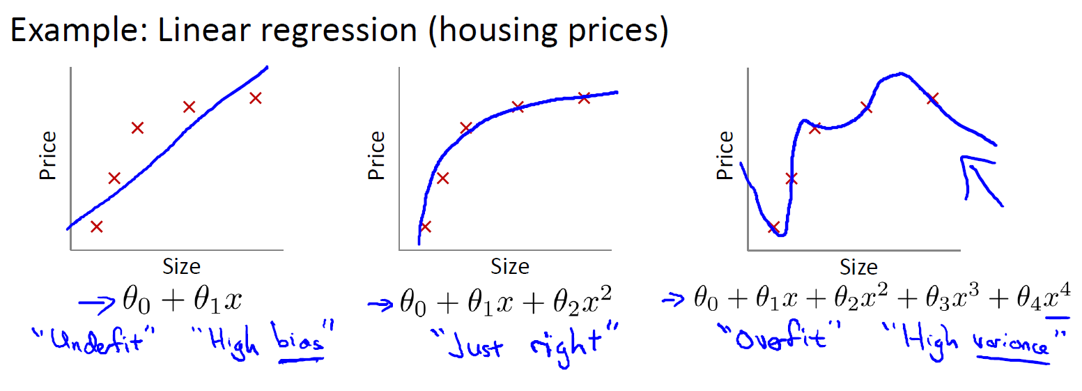
- 第一个模型是一个线性模型,欠拟合(高偏差 high bias),不能很好地适应我们的训练集。它认为房屋的价格会随着size呈线性变化,但是实际上是不会的。
- 第三个模型是一个四次方的模型,过于强调拟合原始数据,而丢失了算法的本质:预测新数据。若给出一个新的值使之预测,它将表现的很差,是过拟合(高方差 high variance),虽然能非常好地适应我们的训练集但在新输入变量进行预测时可能会效果不好;
- 中间的模型似乎最合适。
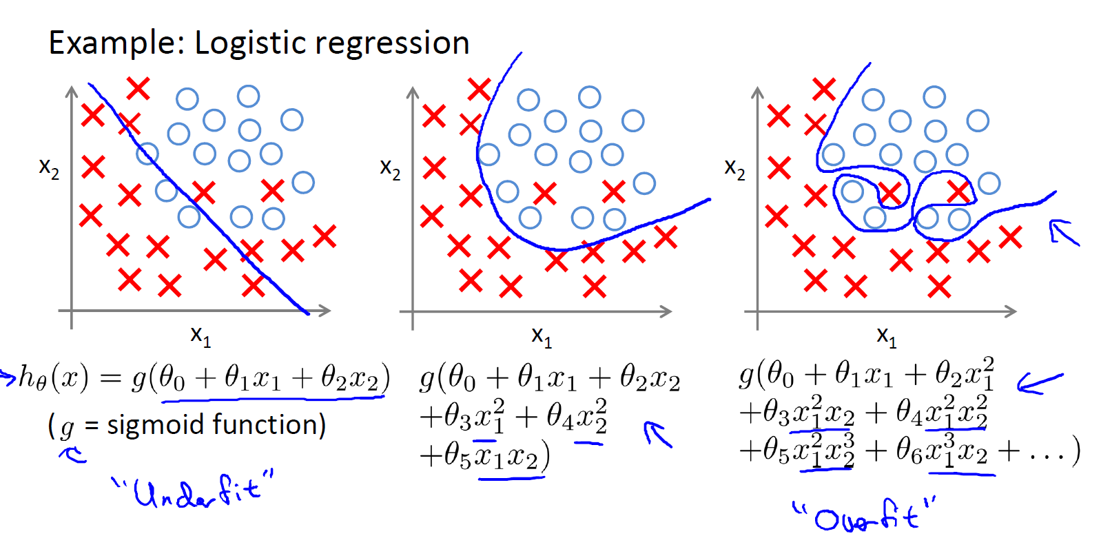
逻辑回归模型中也是同样的问题
Underfitting,or high bias, is when the form of our hypothesis function h maps poorly to the trend of the data.
It is usually caused by a function that is too simple or uses too few features.
overfitting, or high variance, is caused by a hypothesis function that fits the available data but does not generalize well to predict new data. It is usually caused by a complicated function that creates a lot of unnecessary curves and angles unrelated to the data.
过拟合问题的解决方法:
Reduce the number of features:
Manually select which features to keep.
Use a model selection algorithm (比如说PCA).Regularization
Keep all the features, but reduce the magnitude of parameters $\theta_{j}$
Regularization works well when we have a lot of slightly useful features.
也就是说,使用Regularization方法,我们可以保留所有的特征(这些特征对模型训练尽管不是起着关键作用,但是也能做出一定的贡献),又同时能解决过拟合问题
cost function
线性回归中我们发生过拟合的模型是:
$h_{\theta}(x) = \theta_{0} + \theta_{1}x + \theta_{2}x^{2} + \theta_{3}x^{3} + \theta_{4}x^{4}$
如果我们penalize $\theta_{3},\theta_{4}$ 并且让他们非常的小,那么我们的拟合曲线就会变得是一个最高次为2的曲线(3,4次由于系数为0将会变得忽略不计)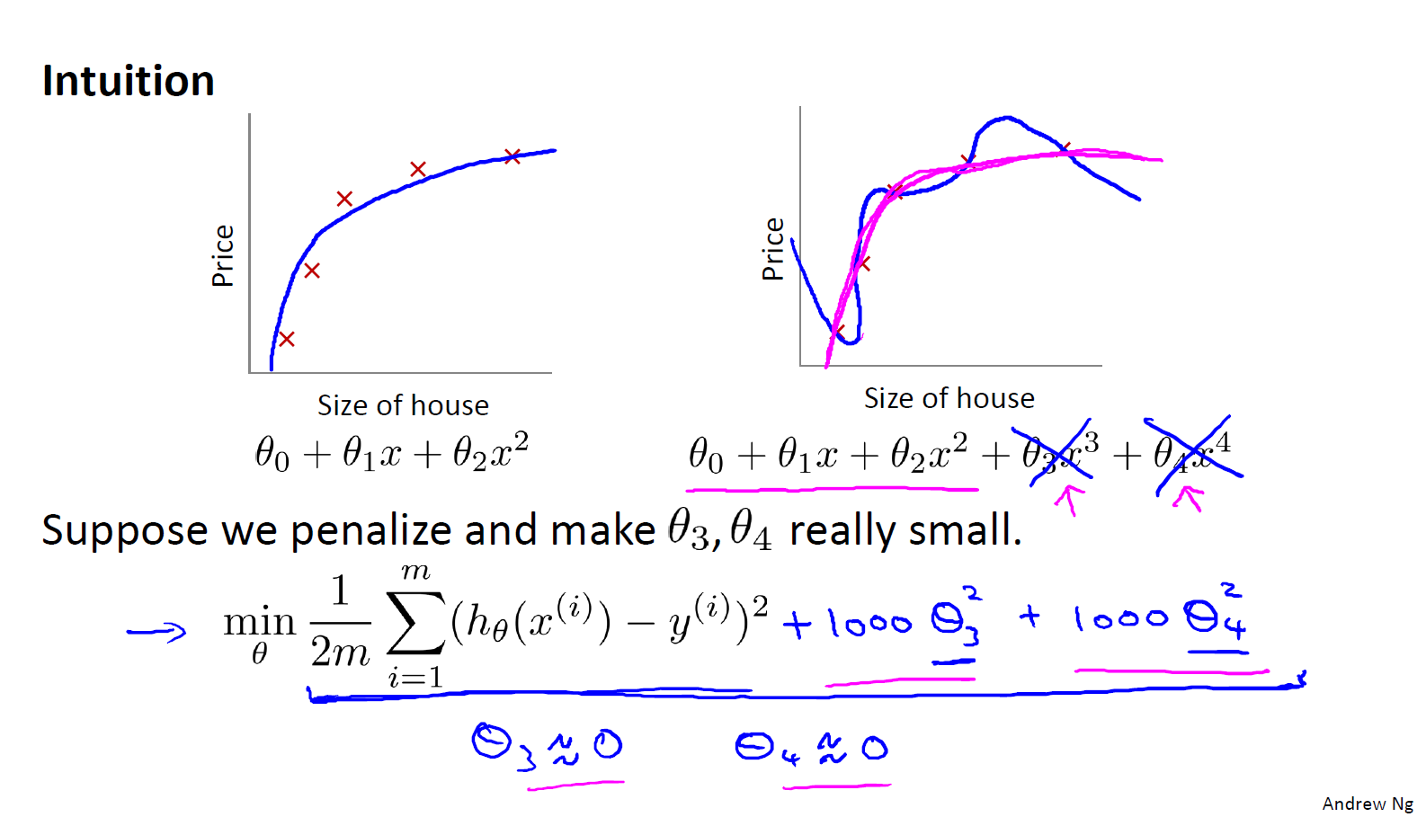
如上图,这样我们的曲线将会更加的光滑,不容易发生过拟合
所以如果我们将$\theta_{j}$加入我们的cost function,然后来最小化我们的cost时,就会同时最小化我们的$\theta_{j}$
下面是cost function的重新定义:
$J\left( {\theta_{0}},{\theta_{1}}…{\theta_{n}} \right)=\frac{1}{2m} [\sum_{i=1}^{m}(h_{\theta }(x^{(i)})-y^{(i)})^{2} + \lambda \sum_{j=1}^{n}\theta_{j}^{2}]$
根据习惯,我们将从$\theta_{1}$开始惩罚,而不是$\theta_{0}$
也就是说,我们在原来的cost上面加了一个$\lambda \sum_{j=1}^{n}\theta_{j}^{2}$(正则项),通过优化cost,我们也会让$\theta_{j}$更小,进而$h_{\theta}(x)$也会更加光滑(可以从前面$\theta_{3},\theta_{4}$的例子上直观感受到)
具体来说,如果我们令 λ 的值很大的话,为了使cost尽可能的小,所有的$\theta$值(不包括$\theta_{0}$)都会在一定程度上减小。
但若$\theta$的值太大了所有的 $\theta$值(不包括$\theta_{0}$),都会趋近于0,这样我们所得到的只能是一条平行于x轴的直线($h_{\theta}(x)=\theta_{0}$),这样我们的模型就会有过强的bias,有过高的偏差,认为预测的价格一直都是等于$\theta_{0}$,换句话说,过大的$\lambda$平滑了太多的$h_{\theta}(x)$,导致了欠拟合(underfitting)
所以对于正则化,我们要取一个合理的$\lambda$的值,这样才能更好的应用正则化
$\lambda$在这里是用来平衡我们的两个不同目标:
- 让我们的模型能够更好的拟合数据
- 同时让我们的$\theta_{j}$更小,来平滑$h_{\theta}(x)$,进而避免过拟合
$\lambda$是rugularization parameter,它决定了我们的参数成本将被扩大到多少
也就是说,我们通过在cost中增加额外的正则项(参数成本),使得$h_{\theta}(x)$变得平滑(减少$h_{\theta}(x)$中某些项的权重),而没有减少特征数目或者改变$h_{\theta}(x)$的形式进而避免过拟合
regularized logistic regression
$J(\theta) = \frac{1}{m}\sum_{i=1}^{m}[-y^{i}log(h_{\theta}(X^{(i)}))-(1-y^{i})log(1-h_{\theta}(x^{(i)}))] + \frac{\lambda}{2m} \sum_{j=1}^{n}\theta_{j}^{2}$
其梯度定义为:
$\frac{\partial J(\theta)}{\partial \theta_{0}} = \frac{1}{m}\sum_{i=1}^{m}(h_{\theta}(x^{(i)})-y^{(i)})x_{0}^{(i)}$
$\frac{\partial J(\theta)}{\partial \theta_{j=1,2…n}} = \frac{1}{m}\sum_{i=1}^{m}(h_{\theta}(x^{(i)})-y^{(i)})x_{j}^{(i)} + \frac{\lambda}{m}\theta_{j}$
那么如果使用梯度下降的话,
Grandient Descent:
repeat{
$\theta_{j} := \theta_{j} - \alpha \cdot \frac{\partial J(\theta)}{\partial \theta_{j}} $
}
依旧是上面这个,但是需要注意$\theta_{0}$是没有正则化项的
python代码实现
这部分,我们使用加入正则项提升逻辑回归算法,正则化是cost函数中的一个术语,它使算法更倾向于“更简单”的模型(在这种情况下,模型将更小的系数)。有助于减少过拟合,提高模型的泛化能力。
设想你是工厂的生产主管,你有一些芯片在两次测试中的测试结果。对于这两次测试,你想决定是否芯片要被接受或抛弃。为了帮助你做出艰难的决定,你拥有过去芯片的测试数据集,从其中你可以构建一个逻辑回归模型
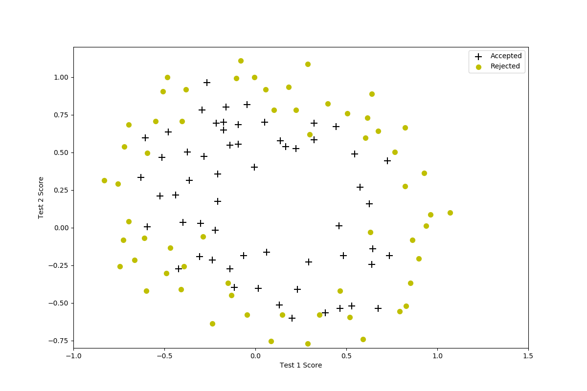
读入数据并可视化
1 | def plotData(data2): |
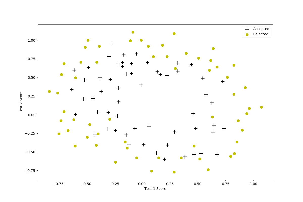
这个数据比第一个练习的复杂得多,没有线性决策边界来的分开两类数据
Feature Mapping
如上图所示,如果我们直接使用线性回归是没有办法很好的达到好分类效果的,因为逻辑回归只能去找到一个线性决策边界
有一种解决办法是:create more features from each data point(根据输入的数据创造更多的特征),我们使用一个特征映射函数,将数据映射映射到所有的多项式项中,最高可达到六次幂
$mapFeature(x) = \begin{bmatrix}
1
\\
x_{1}
\\
x_{2}
\\
x_{1}^{2}
\\
x_{1}x_{2}
\\
x_{2}^{2}
\\
x_{1}^{3}
\\
x_{1}^{2}x_{2}
\\
x_{1}x_{2}^{2}
\\
x_{2}^{3}
\\
…
\\
x_{1}x_{2}^{5}
\\
x_{2}^{6}
\end{bmatrix}
$
通过这样的映射,我们的特征向量,原本只有2D,被转换为了28D的向量。这样我们的逻辑回归分类器通过训练更高维的特征向量,将会有更加复杂的决策边界(非线性)
下面是特征映射函数的实现:1
2
3
4
5
6
7
8
9
10
11
12
13
14
15
16
17
18
19
20
21def mapFeature(x1,x2,degree=6):
# degree = 6
data = {}
for i in range(1,degree+1):
for j in range(0,i+1):
# data2['F'+str(i)+str(j)] = np.power(x1,i-j)*np.power(x2,j)
data["f{}{}".format(i - j, j)] = np.power(x1, i - j) * np.power(x2, j)
data = pd.DataFrame(data)
data.insert(0,'Ones',1)
return data
degree = 6
x1 = data2['Test 1']
x2 = data2['Test 2']
X2 = np.array(mapFeature(x1,x2,degree))
y2 = np.array(data2.iloc[:,2:3])
theta2 = np.zeros(X2.shape[1])
lambdaa = 1
# lambdaa = 100
print(X2[0:5])
print(y2[0:5])
通过这个函数,我们的第一个数据将会是:1
2
3
4
5
6
7[ 1.00000000e+00 5.12670000e-02 6.99560000e-01 2.62830529e-03
3.58643425e-02 4.89384194e-01 1.34745327e-04 1.83865725e-03
2.50892595e-02 3.42353606e-01 6.90798869e-06 9.42624411e-05
1.28625106e-03 1.75514423e-02 2.39496889e-01 3.54151856e-07
4.83255257e-06 6.59422333e-05 8.99809795e-04 1.22782870e-02
1.67542444e-01 1.81563032e-08 2.47750473e-07 3.38066048e-06
4.61305487e-05 6.29470940e-04 8.58939846e-03 1.17205992e-01]
具有28个维度
计算代价函数和梯度
sigmoid函数在第一个练习中已经实现了,现在我们需要做的,是更新代价函数和梯度,加入正则化项。
$J(\theta) = \frac{1}{m}\sum_{i=1}^{m}[-y^{i}log(h_{\theta}(X^{(i)}))-(1-y^{i})log(1-h_{\theta}(x^{(i)}))] + \frac{\lambda}{2m} \sum_{j=1}^{n}\theta_{j}^{2}$1
2
3
4
5
6
7def costFunction(theta,X,y,lambdaa):
h = sigmoid(X.dot(theta.T))
J =(- y.T .dot(np.log(h))-(1-y).T.dot(np.log(1-h) ))/len(X)
reg = theta[2:].T .dot(theta[2:] )* lambdaa / (2*len(X))
J = J + reg
return J
$\frac{\partial J(\theta)}{\partial \theta_{0}} = \frac{1}{m}\sum_{i=1}^{m}(h_{\theta}(x^{(i)})-y^{(i)})x_{0}^{(i)}$
$\frac{\partial J(\theta)}{\partial \theta_{j=1,2…n}} = \frac{1}{m}\sum_{i=1}^{m}(h_{\theta}(x^{(i)})-y^{(i)})x_{j}^{(i)} + \frac{\lambda}{m}\theta_{j}$
1 | def gradFunction(theta,X,y,lambdaa): |
predict
1 | def predict(theta,X): |
算出来的结果为:1
accuracy = 83.05%
decision boundary
下面代码有些不好理解:1
2
3
4
5
6
7
8
9
10
11
12
13
14
15
16
17
18
19
20
21
22#返回num个均匀分布的样本,在[start, stop]
x = np.linspace(-1, 1.5, 250)
# [X,Y] = meshgrid(x,y)
# 将向量x和y定义的区域转换成矩阵X和Y,
# 其中矩阵X的行向量是向量x的简单复制,而矩阵Y的列向量是向量y的简单复制
# 假设x是长度为m的向量,y是长度为n的向量,则最终生成的矩阵X和Y的维度都是 nm(注意不是mn)
xx, yy = np.meshgrid(x, x)
#下面计算这250个点的z值(也就是等高线的z值,z值相同的连成线,就可以形成边界)
z = np.array(mapFeature(xx.ravel(), yy.ravel(), 6))
#上面的xx.ravel()和yy.ravel()都是250*250=62500维度的向量,将他们映射为(62500,28)
z = z @ theta_min # z是(62500,1)
z = z.reshape(xx.shape)
#reshape后,变成了(250,250),这样相当于有250个点的z值
plotData(data2)
# contour画出等高线
plt.contour(xx, yy, z, 0)
plt.ylim(-.8, 1.2)
plt.show()
画出来的决策边界长下面这样:
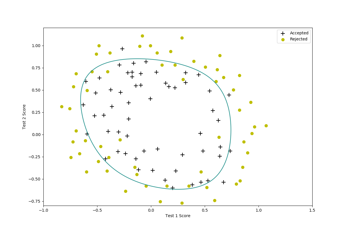
上图是$\lambda=1$
我们还可以尝试使用不同的$\lambda$来看看效果:
- $lambda=0$
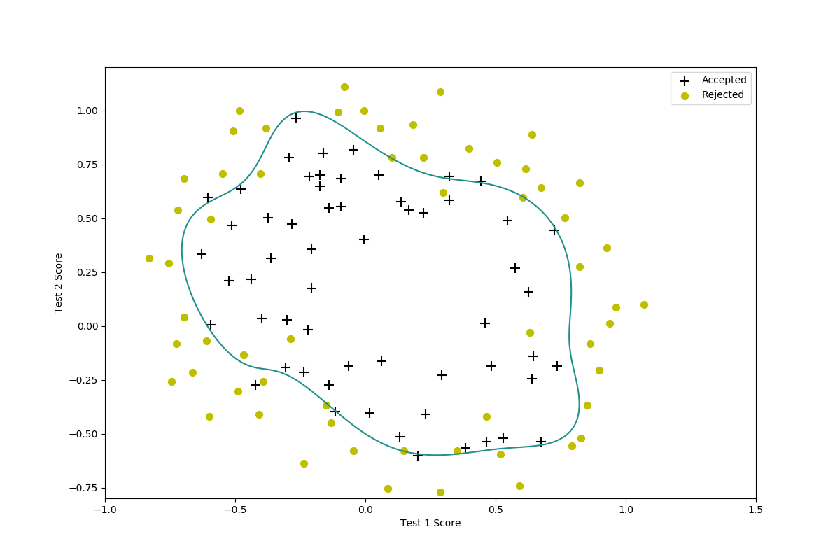
这是我们没有正则化的结果(过拟合)
$lambda=100$
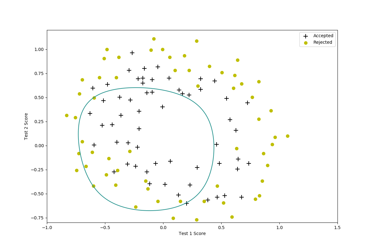
$lambda=1000$
当$lambda=100$否则$lambda=1000$ 实际上已经发生了欠拟合。
完整代码
1 | import numpy as np |